palette = ({
  naipca_iab: "#18557f", complete: "#18557f",
  qz_ipca: "#8a6a1a",
  ipca: "#6f9cc0", rp_pca: "#7a7a7a", ff5: "#b3b3b3",
  naipca_beta_only: "#8a8378", beta_only: "#8a8378",
  band: "rgba(0,0,0,0.06)", muted: "rgba(0,0,0,0.6)", rule: "rgba(0,0,0,0.1)"
})
LANG = (document.documentElement.lang || "en").startsWith("zh") ? "zh" : "en"
STR = ({ en: { view: "View", cost: "Cost (bp per traded dollar)", universe: "Universe", sample: "Sample (months)", log: "Log scale", models: "Models", statistic: "Statistic", theme: "Theme", sort: "Sort by", method: "Method", scenario: "Scenario", block: "Block (months)", metric: "Metric", intervals: "Intervals", cost_bp: "One-way cost (bp)", failed: "Interactive data failed to load. The static figure is shown instead." },
        zh: { view: "视图", cost: "成本(每交易一美元,基点)", universe: "股票池", sample: "样本(月)", log: "对数坐标", models: "模型", statistic: "统计量", theme: "主题", sort: "排序", method: "方法", scenario: "情景", block: "块长(月)", metric: "指标", intervals: "区间", cost_bp: "单边成本(基点)", failed: "交互数据加载失败,改为显示静态图。" } })
t = (k) => STR[LANG][k] ?? STR.en[k] ?? k
fmt2 = (x) => (x == null || Number.isNaN(x)) ? "n/a" : x.toFixed(2)
fmt1 = (x) => (x == null || Number.isNaN(x)) ? "n/a" : x.toFixed(1)
fmtBp = (x) => (x == null || Number.isNaN(x)) ? "> 500" : `${Math.round(x)} bp`
parseMonth = (s) => new Date(`${s}-01T00:00:00Z`)
// Sharpe, annualised, sample std (ddof = 1): matches the release convention
sharpe = (r) => {
  const n = r.length, m = r.reduce((a, b) => a + b, 0) / n
  const v = r.reduce((a, b) => a + (b - m) ** 2, 0) / (n - 1)
  const vol = Math.sqrt(v) * Math.sqrt(12)
  return vol > 1e-12 ? (m * 12) / vol : NaN
}
netSeries = (r, to, bp) => r.map((x, i) => x - to[i] * bp / 1e4)
wealthPath = (r) => { let w = 1; return r.map((x) => (w *= 1 + x)) }
nberMarks = (nber) => Plot.rectX(nber, { x1: (d) => parseMonth(d.start), x2: (d) => parseMonth(d.end), fill: palette.band })A Geometric Framework for Identification in Characteristic-Based Factor Models
Which ruler should a factor model use to tell two combinations of firm characteristics apart?
SSRN preprint, March 2026 (preliminary version) · DOI 10.2139/ssrn.7013178 (listed on SSRN under Yang Liu) · earlier, broader version of Characteristic-Space Metrics · grows out of the PhD thesis
Investors describe each stock by dozens of traits, many of them near-copies of one another. Before a model can say which combinations of traits earn a risk premium, it must decide when two combinations are genuinely different. The paper takes the ruler for that decision from the data and rebuilds instrumented principal component analysis (IPCA) on it. In simulations calibrated to U.S. stocks, with the true priced directions placed by design where characteristics vary most, the rebuilt estimator (NA-IPCA) recovers them. On a distance scale from 0 (exact recovery) to about 1.73 (entirely wrong), NA-IPCA scores 0.01 and an IPCA benchmark with no intercept block (no room for expected return that no factor explains) scores 0.73 (Table 8, p. 38). The simulated returns contain an intercept component, so the comparison does not isolate the ruler.
1 The question
In the agenda, this paper asks the first question: which ruler? The next paper, Characteristic-Space Metrics, asks: once the ruler is chosen, what does it decide, and how precisely?
Firm characteristics overlap and differ in spread. Which combinations of them are genuinely distinct sources of priced risk, and which are only near-copies or leftovers?
To say how much of a stock’s expected return each driver explains, a model must first decide when two combinations of characteristics are really different, and how large each one is. The rule it uses for that is the ruler. Give each characteristic a weight and add them up: every stock gets a score. Such a weighted combination is called a direction (it is not a portfolio). The plain ruler (the Euclidean or identity metric) judges a direction by its weights alone. The characteristic ruler (the Gram metric) judges it by the scores it gives real stocks: how large they typically are, and whether two directions’ scores line up across stocks, high on the same stocks and low on the same stocks.
The ruler, then, is the convention a model uses to measure how large a direction is and how much two directions overlap. Two value signals that pick out the same cheap stocks count as overlapping under the characteristic ruler but as unrelated under the plain ruler.
Standard methods such as principal component analysis (PCA), IPCA (Kelly et al. 2019) and many machine-learning estimators of the stochastic discount factor use the plain ruler (Section 1.1, p. 2); in IPCA, characteristics decide how strongly each stock moves with the common drivers.
The paper’s model has three blocks: hidden factors inferred from the data, observed factors such as the market, and the intercept. The intercept is the part of expected return that no factor in this model explains (the home page’s “alpha” is a close relative, measured against a stated benchmark model).
The answer in one sentence. Measure combinations with the characteristic ruler, taken from how characteristics spread and overlap across stocks; in simulations calibrated to U.S. stocks, with the true priced directions placed by design where characteristics vary most, the estimator built on this ruler (NA-IPCA) recovers them and an IPCA benchmark with no intercept block does not.
2 Why it matters
The ruler decides what counts as “different”. Under the plain ruler, a model can split one priced direction into two factors, let a hidden factor copy an observed benchmark factor already in the model, or push priced content into the intercept (Section 1.1, pp. 2–3).
- Practical. The paper argues that its ruler stops hidden factors from merely reproducing benchmark portfolios, giving users such as portfolio managers a sharper line between priced structure, benchmark exposure and residual noise (Sections 1.4–1.5, pp. 5–6). This is argued and simulated, not shown on live portfolios.
- Statistical. A good fit does not reveal the right structure: in the paper’s metric sweep (Table 1 below), IPCA fits returns better than NA-IPCA while missing the true directions (Table 9, p. 42).
3 The argument at a glance
- Question. Stocks are described by dozens of characteristics, many of them versions of a few traits (Section 6.2, p. 28). → The question
- Why. Because of this overlap, the plain ruler that PCA and IPCA use misjudges which combinations are truly different (Section 1.1, p. 2). → Why it matters
- Framework. Estimate the characteristic ruler from the data and write all the model’s rules in it, including how the three blocks are kept apart and how much the intercept may carry. The result is NA-IPCA. → The framework
- Mechanism. Directions that look unrelated under the plain ruler can overlap under the characteristic ruler, so separating the blocks with the characteristic ruler stops double counting. → A simple example
- Evidence. The U.S. characteristic ruler is strongly uneven. In the headline simulation NA-IPCA recovers the priced directions and an IPCA benchmark with no intercept block misses them, so the comparison does not isolate the ruler. IPCA comes close to the true directions (0.01–0.06) in the stress-test designs (Tables 17–19). It stays far off (0.73–0.99) in the metric sweep (Table 1 below) and in the correlation sweep, which moves characteristics from unrelated toward the U.S. pattern (Table 10, p. 43). → Design and main results
- Contribution. The ruler becomes an explicit, estimated part of the model’s economics. → How it relates to prior work
- Boundary. The paper does not test NA-IPCA on real returns or portfolios; a real-data application is left to a separate study (pp. 50–51). → Scope
4 The framework
Let Z_t hold L characteristics for the N_t stocks observed in month t. The characteristic ruler is the long-run average of how characteristics spread and move together across stocks (Section 2, p. 6):
Q_Z = \frac{1}{T}\sum_{t=1}^{T} \frac{1}{N_t} Z_t^{\top} Z_t .
Under this ruler, the size of a direction with weights a is (a^{\top} Q_Z a)^{1/2}: roughly, how widely the scores it gives stocks vary. The plain ruler replaces Q_Z with the identity matrix.
Expected excess returns are split into the three blocks (Section 2, p. 7):
\mathbb{E}_t\!\left[r_{t+1}\right] = Z_t\left(\Gamma_\beta f_t + \Gamma_\delta F^{\text{obs}}_t + \Gamma_\alpha\right).
\Gamma_\beta holds the loadings on the hidden factors f_t, \Gamma_\delta the loadings on observed factors such as traded benchmarks, and \Gamma_\alpha is the intercept, built from characteristics (Table 1, p. 7). The estimator, No-Arbitrage IPCA (NA-IPCA), states the rules for all three blocks in terms of Q_Z and caps how much the intercept may carry. The cap is the “no-arbitrage” in the name: the tighter it is, the closer the model comes to strict no-arbitrage (Section 2, p. 8). With the plain ruler and an intercept cap so loose that it has no effect, NA-IPCA reduces to IPCA (p. 22).
For specialists: the restrictions, the estimator and the inference
In Q_Z, the latent loadings are orthonormal, \Gamma_\beta^{\top} Q_Z \Gamma_\beta = I; the observed and intercept blocks are Q_Z-orthogonal to the latent span; and the intercept’s size is capped, \psi(\Gamma_\alpha) = \Gamma_\alpha^{\top} Q_Z \Gamma_\alpha \le \delta (Section 2, pp. 7–8). NA-IPCA is weighted least squares restricted to this set (Proposition 3.1, p. 14), with rotation-invariant asymptotic inference for the identified spans (Section 4, from p. 17).
5 A simple example
Take two characteristics, A and B, say two versions of value, that move together across stocks with correlation ρ. The priced direction uses both equally. Suppose a model puts A in one block and B in another. Under the plain ruler A and B look unrelated, so each block claims the shared part.
Try this. (1) Set ρ to 0: both splits explain 100% between them. (2) Raise ρ to 0.9: split with the plain ruler, the two blocks claim 190%. What to notice. Split with the characteristic ruler, the total always stays at 100%, because block B keeps only what block A leaves unexplained. The shared part is counted once.
Figure 1: Two rulers for two correlated characteristics. Illustrative numbers, not the paper’s data.
How to read it. Left: the weights that define A and B (gold) and the priced direction (dark). Directions of size 1 lie on the dashed circle under the plain ruler and on the blue ellipse, a^{\top} Q a = 1, under the characteristic ruler (Q has 1 on the diagonal and ρ off it). Right: the share of the priced direction each block explains, both rows scored with the characteristic ruler, since a direction reaches returns only through the scores it gives stocks: (1+\rho)/2 for A or B alone, (1-\rho)/2 for B net of A. The toy’s ρ is a correlation between two characteristics, not the weight ρ in the paper’s correlation sweep (Table 10, p. 43). Source: illustrative calculation built on the paper’s definitions (Section 2; Figure 3, p. 34); no data file.
6 Design and main results
The paper estimates the characteristic ruler on the replication panel of Kelly et al. (2019): 37 characteristics including a constant, 12,813 firms, July 1964 to May 2014 (Section 6.1, p. 27; Table 2, p. 28). It then simulates 1,000 stocks over 240 months, 300 times, with characteristics drawn to match this ruler. By design, the three hidden factors sit where characteristics vary most, the two observed factors are deliberately weak, and the returns contain a nonzero intercept component (Section 7.1, pp. 34–36; Table 7, p. 36). Same simulated data, three estimators: NA-IPCA, an IPCA benchmark with no intercept block, and PCA (Section 7.2, p. 36).
Figure 2: The characteristic ruler is strongly uneven. Share of the total spread carried by each of the 15 largest directions of Q_Z.
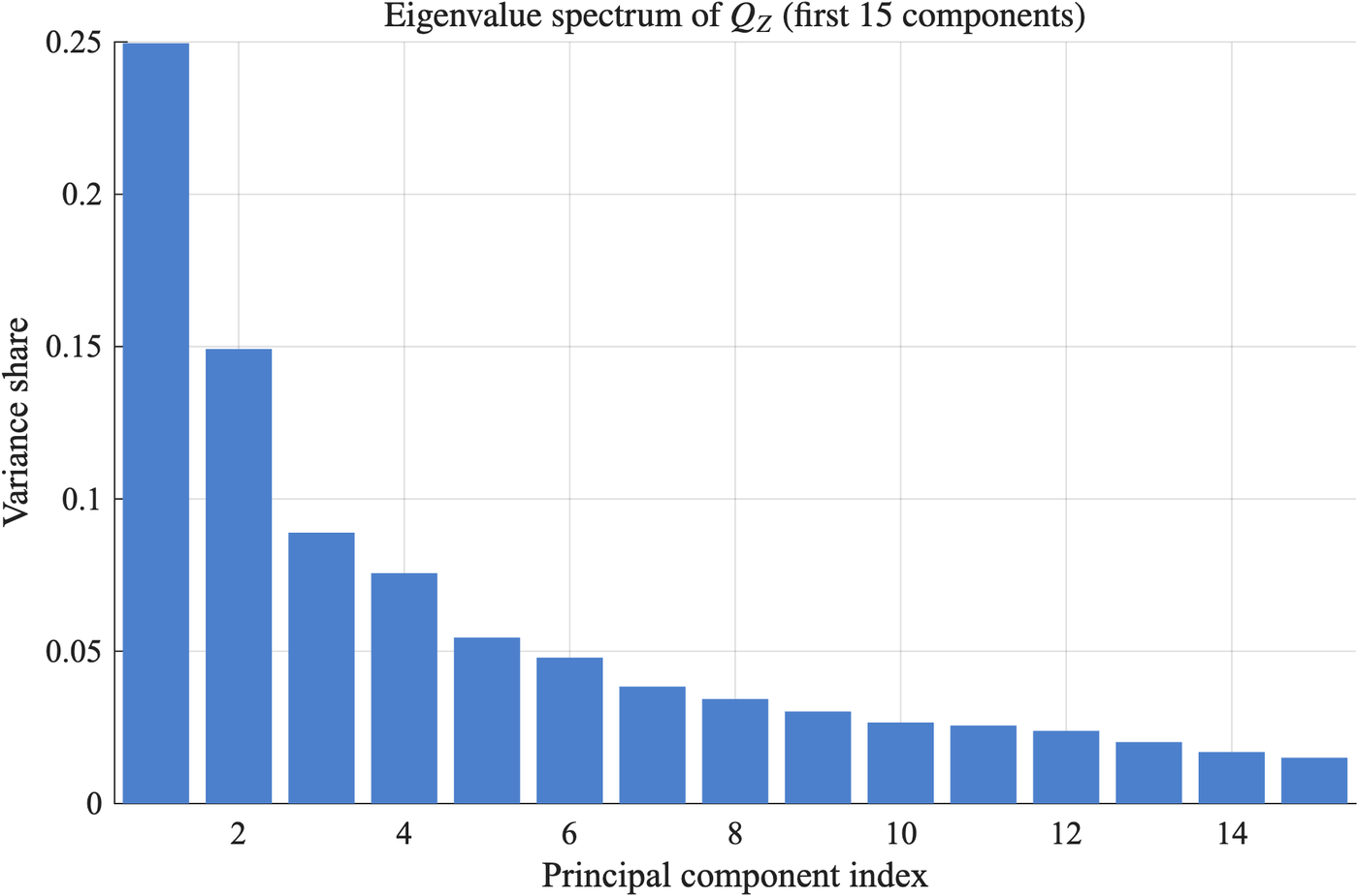
How to read it. Each bar is one of the 37 directions of Q_Z, largest first. Source: SSRN preprint, March 2026, Figure 2, p. 33 (reproduced from the paper). Paper page
What this shows. One of the 37 columns is a constant (Table 6, p. 32); its entry of 1 in a total of 4.01 matches the largest eigenvalue (Table 7, p. 36), so the 25% first bar is essentially that constant. The unevenness is in the rest: if the other 36 were unrelated and equally spread, as the plain ruler assumes, each would carry about 2%; the next four carry about 37% between them (Table 5, p. 30). This describes how characteristics overlap, not which directions are priced.
Figure 3: In the headline simulation, NA-IPCA finds the true latent span; IPCA without an intercept block and PCA do not. Distance between the estimated and the true factor directions (the “span”).
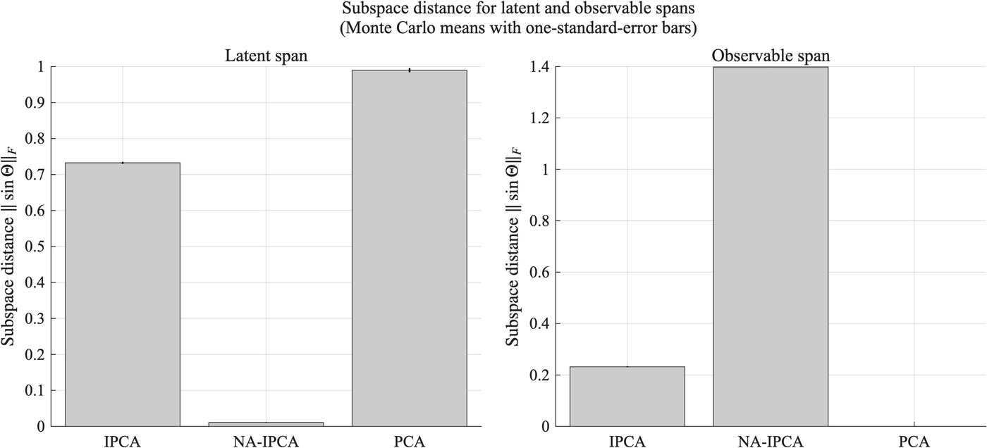
How to read it. Left panel (“latent”): hidden factors; right panel (“observable”): observed factors. The distance, \lVert \sin\Theta \rVert_F, is 0 for exact recovery and reaches its maximum when the estimated directions are entirely wrong: \sqrt{3} \approx 1.73 for the three hidden-factor directions and \sqrt{2} \approx 1.41 for the two observed-factor directions (footnote 10, p. 39). On the observed block the ranking reverses: IPCA 0.23, NA-IPCA 1.40, almost the maximum, so NA-IPCA misses the observed-factor directions. PCA has no observed block, so its right-panel bar is missing, not zero. The paper reads this as the design’s doing: the observed factors were made deliberately weak (Section 7.2, p. 37). Source: SSRN preprint, March 2026, Figure 4, p. 39, and Table 8, p. 38 (reproduced from the paper). Paper page
What this shows. On the scale from 0 to about 1.73, and with the priced directions placed by design where characteristics vary most, NA-IPCA’s hidden-factor directions sit 0.011 from the truth. Those of the IPCA benchmark with no intercept block sit 0.73 away, and those of PCA 0.99 away (Table 8, p. 38). On an overlap measure where 0 means fully separated blocks, the IPCA benchmark’s hidden and observed blocks overlap by 0.069; NA-IPCA, which keeps them apart by construction, scores 0.0005. The toy’s double counting appears here in a milder form.
Table 1: Change only how characteristics are distributed (the paper’s metric sweep). True loadings and factors fixed; four ways of drawing the characteristics; Monte Carlo means over 300 replications (Table 9, p. 42).
| Characteristic geometry | Latent distance, IPCA | Latent distance, NA-IPCA | Overlap, IPCA | Overlap, NA-IPCA | In-sample R², IPCA | In-sample R², NA-IPCA |
|---|---|---|---|---|---|---|
| Empirical Q_Z | 0.7325 | 0.0112 | 0.0663 | 0.0005 | 0.9588 | 0.5827 |
| Identity | 0.9843 | 0.0075 | 0.0463 | 0.0008 | 0.9449 | 0.1601 |
| Q_Z, eigenvectors permuted | 0.9907 | 0.0387 | 0.0401 | 0.0017 | 0.9885 | −0.0735 |
| Q_Z, spectrum flattened | 0.9831 | 0.0073 | 0.0466 | 0.0008 | 0.9453 | 0.1579 |
Latent distance: \lVert \sin\Theta_\beta \rVert_F for the hidden-factor directions, 0 to about 1.73. Overlap: hidden–observed block overlap in Q_Z. R²: in-sample panel R² of returns. Source: SSRN preprint, March 2026, Table 9, p. 42.
What this shows. In every row the true directions sit, by design, where characteristics vary most in the U.S. data (Section 7.3, p. 38). The IPCA benchmark stays 0.73–0.99 from the truth; NA-IPCA stays at or below 0.04. In the Identity and spectrum-flattened rows the characteristics are drawn unrelated and equally spread, so their characteristic ruler is the plain ruler up to scale (footnote 9, pp. 38–39), yet the gap is just as large: it does not come from uneven characteristics. IPCA still fits returns better in every row, with an R² of 0.94–0.99 against at most 0.58 for NA-IPCA (Table 9, p. 42). In the paper’s stress-test designs, where the intercept component is about 0.05 in size against 0.50 in the headline design, IPCA comes close to the true directions, 0.01–0.06 away (Tables 17–19, pp. 63–64).
7 How it relates to prior work
The table lists the closest reference points (Section 1.2, pp. 3–4).
| Prior work | What it established | What this paper adds |
|---|---|---|
| Approximate factor models (Bai and Ng 2002) | How many common factors a large panel has, under weak dependence | Once the number is set, asks which directions are priced, measured with an estimated ruler |
| IPCA (Kelly et al. 2019) | Characteristics instrument time-varying betas; the model admits an intercept and observed factors and tests whether each is zero | Writes the model’s scale and block separation with the characteristic ruler and caps how much the intercept may carry |
| RP-PCA, risk-premium PCA (Lettau and Pelger 2020) | Adding a pricing-error penalty to PCA gives factors that also fit average returns | Puts pricing discipline into the set of admissible models, through the ruler and the intercept cap |
| Shrinking the cross-section (Kozak et al. 2020) | A prior that shrinks the stochastic discount factor’s coefficients on characteristic portfolios, most strongly along their low-variance principal components | Uses the characteristic ruler not as a penalty but to set the model’s scale and keep its blocks apart |
The simulations’ weak observed factors follow work on weak and spurious factors (Bryzgalova 2015; Kozak et al. 2018) (p. 32); the intercept cap is related to volatility bounds (Hansen and Jagannathan 1991) (p. 10).
Much prior work first extracts factors with a fixed ruler and then adds pricing restrictions on top (Section 1.2, p. 4). This paper makes the ruler itself something to estimate. The tools are known; what is new is an estimator and inference built on that estimated ruler.
This is the earliest paper in the agenda to set out the idea that runs through it: take the ruler from the data, and write the model’s rules in it. Characteristic-Space Metrics states the ruler’s role precisely: it decides the split, not the fit, and its estimation error belongs in the standard errors. Interpreting Pricing Errors holds the ruler fixed to read alphas fairly. Characteristic Geometry shows that the ruler’s units can move portfolios while forecasts barely move; the job market paper shows that the way the library is written can move holdings with no new information.
8 Scope
- The paper does not test NA-IPCA on real returns or portfolios. In its simulations, out-of-sample fit is the same for both estimators (Table 19, p. 64); a full out-of-sample application in U.S. equities is left to a separate study (Section 8, pp. 50–51).
- In the simulations the true priced directions sit, by design, where characteristics vary most, and the IPCA benchmark lacks the intercept block that the simulated returns contain (Sections 7.1–7.2, pp. 34–36). So the comparison does not isolate the ruler, and it cannot tell which ruler real markets follow.
- The characteristic ruler is estimated from one sample, 1964 to 2014. If the distribution of characteristics shifts, the ruler should be re-estimated (Section 8, p. 50).
- The intercept is a capped part of expected returns that the factors leave unexplained. It is not a measured mispricing.
- The large-sample theory holds only under the conditions the paper states. Its efficiency result is local: among estimators that respect the paper’s restrictions, NA-IPCA reaches the efficiency bound (Section 4.3, p. 19). The paper does not claim that NA-IPCA is the best estimator in general.
References
Bai, Jushan, and Serena Ng. 2002. “Determining the Number of Factors in Approximate Factor Models.” Econometrica 70 (1): 191–221. https://doi.org/10.1111/1468-0262.00273.
Bryzgalova, Svetlana. 2015. “Spurious Factors in Linear Asset Pricing Models.” Working paper. https://sabryzgalova.com/research/.
Hansen, Lars Peter, and Ravi Jagannathan. 1991. “Implications of Security Market Data for Models of Dynamic Economies.” Journal of Political Economy 99 (2): 225–62. https://doi.org/10.1086/261749.
Kelly, Bryan T., Seth Pruitt, and Yinan Su. 2019. “Characteristics Are Covariances: A Unified Model of Risk and Return.” Journal of Financial Economics 134 (3): 501–24. https://doi.org/10.1016/j.jfineco.2019.05.001.
Kozak, Serhiy, Stefan Nagel, and Shrihari Santosh. 2018. “Interpreting Factor Models.” Journal of Finance 73 (3): 1183–223. https://doi.org/10.1111/jofi.12612.
Kozak, Serhiy, Stefan Nagel, and Shrihari Santosh. 2020. “Shrinking the Cross-Section.” Journal of Financial Economics 135 (2): 271–92. https://doi.org/10.1016/j.jfineco.2019.06.008.
Lettau, Martin, and Markus Pelger. 2020. “Factors That Fit the Time Series and Cross-Section of Stock Returns.” Review of Financial Studies 33 (5): 2274–325. https://doi.org/10.1093/rfs/hhaa020.
Citation
BibTeX citation:
@report{liu2026framework,
  author = {Liu, Mingyang},
  title = {A {Geometric} {Framework} for {Identification} in
    {Characteristic-Based} {Factor} {Models}},
  date = {2026-03},
  url = {https://yl7919.github.io/research/geometric-framework.html},
  doi = {10.2139/ssrn.7013178},
  langid = {en}
}
For attribution, please cite this work as:
Liu, Mingyang. 2026. A Geometric Framework for Identification in
Characteristic-Based Factor Models. SSRN preprint. https://doi.org/10.2139/ssrn.7013178.